Developing the Model

There are many AI model architectures that predict outputs based on input data. But what do they all have in common?

• Data-driven adaptation: All models learn by adjusting their internal representations based on data or interactions with the environment,
• Representation of knowledge: Each method creates some internal structure - weights, rules, clusters, or policies - that encodes what it has learned,
• Feedback mechanism: Every model has a way to evaluate its own performance,
• Generalization: Regardless of whether explicit labels are used, the goal is for the model to perform well on unseen data, not just memorize the training set.

In summary, whether we are talking about supervised, unsupervised, or reinforcement learning, machine learning is about adapting an internal representation to better reflect the data or environment, guided by some measure of success or feedback signal.

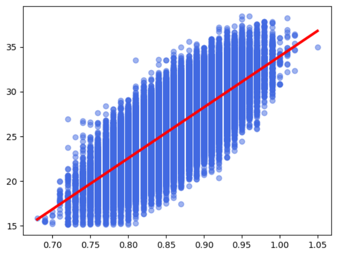
Train for a future reference simple linear regression model

This section can be skipped; just take note of the accuracy of the linear regression model.

import pandas as pd
from sklearn.model_selection import train_test_split
from sklearn.linear_model import LinearRegression
import numpy as np
import matplotlib.pyplot as plt

data = pd.read_csv("/kaggle/input/playground-series-s5e12/train.csv")

# Split a dataset into training and testing sets
X = data["waist_to_hip_ratio"]
y = data["bmi"]

X = X.values
y = y.values

X_train, X_test, y_train, y_test = train_test_split(
    X, 
    y, 
    test_size=0.3, 
    random_state=420
)

# Train for a future reference simple linear regression model
X_train = X_train.reshape(-1, 1)
X_test = X_test.reshape(-1, 1)
y_train = y_train.reshape(-1, 1)
y_test = y_test.reshape(-1, 1)

model = LinearRegression()
model.fit(X_train, y_train)

X_line = np.array([X.min(), X.max()])
y_line = model.coef_[0] * X_line + model.intercept_
fig, ax = plt.subplots()
ax.scatter(X, y, color='royalblue', alpha=0.5)
ax.plot(X_line, y_line, color='red', linewidth=3)

# Calculate accuracy
threshold = 25 # Overweight is defined as a BMI over 25

total = X_test.shape[0]
good_classified = 0
for i in range(total):
    y_true = 1 if y_test[i] > threshold else 0
    pred = 1 if model.predict(X_test[i].reshape(1, -1)) > threshold else 0

    if pred == y_true:
        good_classified += 1

print(f"Accuracy of LinearRegression: {good_classified / total}")

Accuracy of LinearRegression: 0.7834619047619048

What Do We Need?

To build a learning system, we need to go through five fundamental steps (often repeatedly):

1. The task the model should solve – we must clearly define the goal for which the model will be used.
2. Internal state of knowledge – the information the model stores about what it has learned.
3. Applying knowledge – the method that uses the stored knowledge to process input data and generate a response.
4. Feedback mechanism – a method for evaluating whether the model is learning.
5. Update mechanism – a method for modifying the internal state of knowledge based on feedback.

1. The Task the Model Should Solve

The first and key step in creating a model is to clearly define the problem it is intended to solve. Without a clear definition of the task, it will be difficult to determine what and how the model should learn. Designing systems with general intelligence is extremely challenging, so in practice we focus on narrow, well-defined tasks, which allow for a simpler and more controlled representation of knowledge.

2. Internal State of Knowledge

The next step is to decide how knowledge will be stored and what exactly the model should learn. This could be, for example, a set of hyperplane coefficients, a single geometric parameter, or an optimal data partition.

3. Applying Knowledge

The next step is to define how the model uses the stored knowledge to process input data and generate a response, e.g., a prediction. It is important to note that the method of prediction does not have to be tied to the learning process - the model may learn without using predictions and still generate outputs in a different way. A good example of this is the k-means algorithm.

4. Feedback Signal

Next, we need to consider how the model will learn. For this, we must also define how the model will know if its performance is improving. The feedback signal (also called the loss function) does not have to be perfect or exact - its role is simply to indicate a direction of change, e.g., whether the internal representation should be increased, decreased, or modified in another way.

Without a feedback mechanism, the model cannot assess its own progress and therefore cannot learn.

5. Update Mechanism

The final step is to define the update mechanism, which uses the feedback signal to modify the model’s internal state of knowledge. This can be implemented in many ways, depending on how the model’s knowledge is represented.

Designing your own model architecture is an iterative process and typically involves repeatedly moving between these five pillars, gradually refining their form and interrelationships.

The Most Use(less) Predictive Model

As I mentioned earlier, the first step in creating a model is to define the problem it is meant to solve. This will later help determine what and how the model should learn. In my case, the goal is to predict whether a person is overweight (BMI > 25) based on the waist-to-hip ratio (WHR).

I want to create a model that specializes in this task, rather than generally predicting values of y from X (like a standard regression model). This assumption is beneficial because I can be confident that the data will always lie in the first quadrant, since both WHR and BMI are positive. Fortunately, the necessary data has already been collected, so we do not need to worry about that.

The next step is to define what the model should technically learn. This could be, for example, the coefficients of a line as in linear regression, or the optimal data splits as in decision trees.

Our problem can be approached either as a classification task (BMI > 25 → class 1, BMI ≤ 25 → class 0) or as a regression task (predicting the BMI value and then checking whether it exceeds 25). Inspired by regression models, I came up with the idea of teaching the model the angle by which a unit vector [1, 0] anchored at the origin should be rotated (without a parameter for shifting). This introduces additional constraints (the data must be properly rotated and shifted).

Prediction would involve scaling this vector by the X value (hence our training data should be restricted to the range <0,1>). The Y-coordinate of the scaled vector would indicate the predicted value. (With the deep hope that no one will ever have a WHR higher than in the dataset)

The model would learn the angle by treating all points (WHR, BMI) as vectors anchored at the origin. Then, the cosine similarity between them and the model’s vector would be calculated, and the resulting angles would be averaged. The closer the cosine similarity is to 1, the smaller the error made by the model.

The angle is updated only once, by assigning the average angle obtained using the inverse cosine function.

import numpy as np


class MostUselessAlgorithm:
    def __init__(self):
        self.alpha = 0
        self.max_x = 0
    
    def fit(self, X, y):
        angles = []
        # Needed to adjust our vector
        self.max_x = np.max(X)
        
        for j in range(X.shape[0]):
            loss = self._get_loss(X[j], y[j])
            angle = np.arccos(loss)
            angles.append(angle)

        self.alpha = np.mean(angles)
            
    def predict(self, X):
        return np.clip((X * self.get_vector())[1], 0, 1)

    def _get_loss(self, X, y):
        a = np.hstack([X, y])
        b = X * self.get_vector()

        return self._get_cosine_simlarity(a, b)

    def get_vector(self):
        return np.array([np.cos(self.alpha), np.sin(self.alpha)]) * (self.max_x / np.cos(self.alpha))

    def _get_cosine_simlarity(self, a, b):
        dot = np.dot(a, b)
        norm_a = np.linalg.norm(a)
        norm_b = np.linalg.norm(b)

        if norm_a == 0 or norm_b == 0:
            return 0
        
        return dot / (norm_a * norm_b)

# Train
most_useless_algorithm = MostUselessAlgorithm()
most_useless_algorithm.fit(X_train, y_train)

# Visualize
alpha = most_useless_algorithm.alpha
fig, ax = plt.subplots()

vector = most_useless_algorithm.get_vector()

ax.scatter(X_train, y_train, color='royalblue', alpha=0.5)
plt.quiver(0, 0, vector[0], vector[1], angles='xy', scale_units='xy', scale=1, color='red')

# Overweight is defined as a BMI over 25
threshold = 25

total = X_test.shape[0]
good_classified = 0
for i in range(total):
    y_true = 1 if y_test[i] > threshold else 0
    pred = 1 if most_useless_algorithm.predict(X_test[i]) > threshold else 0

    if pred == y_true:
        good_classified += 1

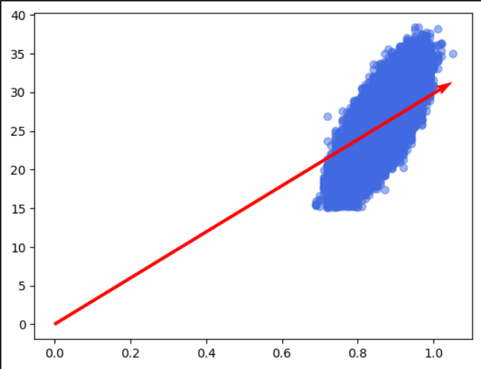
print(f"Accuracy of MostUselessAlgorithm (without rotating): {good_classified / total}")

Accuracy of MostUselessAlgorithm (without rotating): 0.3896809523809524

As we can see, the accuracy of our model is not satisfactory. This is because our vector does not represent the general trend of the data, as the points are not properly rotated and adjusted. To address this, I will adjust the points so that they are correctly rotated and scaled to the range <0, 1>, giving the algorithm a chance to capture the overall trend.

from sklearn.preprocessing import MinMaxScaler

# Scaler X
scaler_X = MinMaxScaler(feature_range=(0, 1))
X_train_scaled = scaler_X.fit_transform(X_train)
X_test_scaled = scaler_X.transform(X_test)

# Scaler y
scaler_y = MinMaxScaler(feature_range=(0, 1))
y_train_scaled = scaler_y.fit_transform(y_train.reshape(-1, 1))
y_test_scaled = scaler_y.transform(y_test.reshape(-1, 1))

# Train
most_useless_algorithm = MostUselessAlgorithm()
most_useless_algorithm.fit(X_train_scaled, y_train_scaled)

# Visualize
alpha = most_useless_algorithm.alpha
fig, ax = plt.subplots()

vector = most_useless_algorithm.get_vector()

ax.scatter(X_train_scaled, y_train_scaled, color='royalblue', alpha=0.5)
plt.quiver(0, 0, vector[0], vector[1], angles='xy', scale_units='xy', scale=1, color='red')

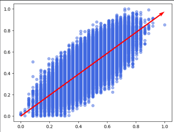
Now, let's see the accuracy that our model achieves.

# Overweight is defined as a BMI over 25
print(scaler_y.transform(np.array(25).reshape(-1, 1)))
threshold = 0.4248927

total = X_test_scaled.shape[0]
good_classified = 0
for i in range(total):
    y_true = 1 if y_test_scaled[i] > threshold else 0
    pred = 1 if most_useless_algorithm.predict(X_test_scaled[i]) > threshold else 0

    if pred == y_true:
        good_classified += 1

print(f"Accuracy of MostUselessAlgorithm: {good_classified / total}")

[[0.4248927]]

Accuracy of MostUselessAlgorithm: 0.7853142857142857

This is a satisfactory level, comparable to the linear regression used at the beginning of this post. Now that we know our algorithm works, let’s focus on optimizing it and improving code clarity. We should consider which operations can be vectorized, which calculations are unnecessarily repeated, and whether we can somehow improve the numerical stability of our algorithm.

import numpy as np


class MostUselessAlgorithmOptimized(MostUselessAlgorithm):
    def __init__(self):
        super().__init__()

    def fit(self, X, y):
        self.max_x = np.max(X)
        angles = self._get_angles(X, y)
        self.alpha = np.mean(angles)

    def predict(self, X):
        return (X * (self.get_vector()[1]))

    def _get_angles(self, X, y):
        angles = np.arctan2(y, X)
        return angles

# Train
most_useless_algorithm_optimized = MostUselessAlgorithmOptimized()
most_useless_algorithm_optimized.fit(X_train_scaled, y_train_scaled)

# Visualize
alpha = most_useless_algorithm_optimized.alpha
fig, ax = plt.subplots()

vector = most_useless_algorithm_optimized.get_vector()

ax.scatter(X_train_scaled, y_train_scaled, color='royalblue', alpha=0.5)
plt.quiver(0, 0, vector[0], vector[1], angles='xy', scale_units='xy', scale=1, color='red')

# Overweight is defined as a BMI over 25
print(scaler_y.transform(np.array(25).reshape(-1, 1)))
threshold = 0.4248927

total = X_test_scaled.shape[0]
good_classified = 0
for i in range(total):
    y_true = 1 if y_test_scaled[i] > threshold else 0
    pred = 1 if most_useless_algorithm_optimized.predict(X_test_scaled[i]) > threshold else 0

    if pred == y_true:
        good_classified += 1

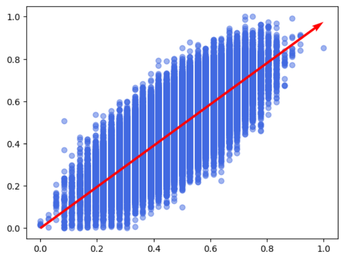
print(f"Accuracy of MostUselessAlgorithm (optimized): {good_classified / total}")

[[0.4248927]]

Accuracy of MostUselessAlgorithm (optimized): 0.7853142857142857

Benchmark:

import time
import numpy as np

def benchmark(func, n_runs=10, *args, **kwargs):
    times = []
    
    for _ in range(n_runs):
        start = time.perf_counter()
        
        func(*args, **kwargs)
        
        end = time.perf_counter()
        times.append(end - start)
    
    median_time = np.median(times)
    return median_time


median_time = benchmark(most_useless_algorithm.fit, 10, X_train_scaled, y_train_scaled)
print(f"Median time (fit, most_useless_algorithm): {median_time:.6f} s")

median_time = benchmark(most_useless_algorithm.predict, 10, X_test_scaled)
print(f"Median time (predict, most_useless_algorithm): {median_time:.6f} s")

median_time = benchmark(most_useless_algorithm_optimized.fit, 10, X_train_scaled, y_train_scaled)
print(f"Median time (fit, most_useless_algorithm_optimized): {median_time:.6f} s")

median_time = benchmark(most_useless_algorithm_optimized.predict, 10, X_test_scaled)
print(f"Median time (predict, most_useless_algorithm_optimized): {median_time:.6f} s")

Median time (fit, most_useless_algorithm): 9.140649 s

Median time (predict, most_useless_algorithm): 0.003036 s

Median time (fit, most_useless_algorithm_optimized): 0.014482 s

Median time (predict, most_useless_algorithm_optimized): 0.000159 s

As you can see, after optimization our model is significantly faster. I vectorized the Python loops, and in the predict function we now multiply only the y-coordinate, not the entire vector by X. Additionally, instead of calculating the cosine similarity and then the angles, we do essentially the same by computing the angles between the vectors and the X-axis and averaging them.

The Most Use(ful) Predictive Model

I’ll leave the development of such a model to you. As you may have noticed, it’s not an easy task and it’s an iterative process. I hope that if you build a state-of-the-art model architecture, you’ll remember your old friend… 😄

Summary

I hope I managed to present the process of designing machine learning algorithms as clearly as possible. The algorithm I presented is not perfect and has many limitations. Designing your own algorithm is very demanding and requires a lot of knowledge and patience, so I will leave this topic to specialists (or to my future self, if I pursue a PhD in AI 😄).

See you in the next post!