

Introduction
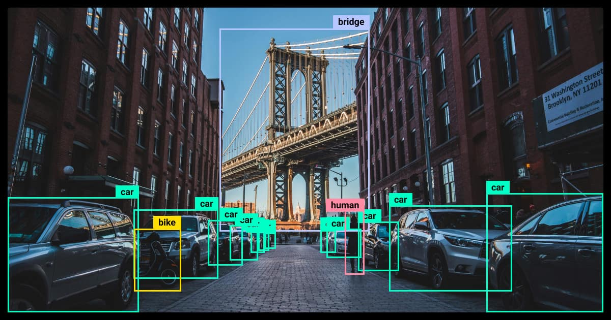
Convolutional neural networks have wide applications in the fields of computer vision, signal processing, and time series analysis. One of the most fascinating applications is computer vision – it gives machines a kind of "sight", enabling them to interact more effectively with the world around us.
A good example is autonomous cars, which are capable of driving on their own. CNNs form part of larger models, which nowadays often also make use of Transformers (Attention Is All You Need).
Advantages of CNNs over Classical Neural Networks
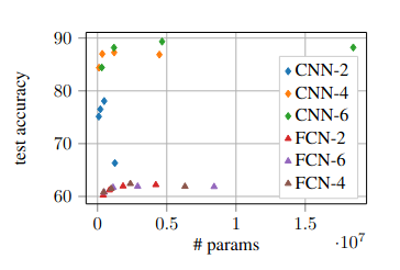
One of the main advantages of CNNs over classical neural networks (fully connected, not combined with another architecture like CNNs) is the smaller number of parameters to learn (while maintaining the same or even better accuracy).
 https://arxiv.org/pdf/2010.01369
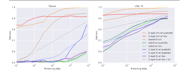
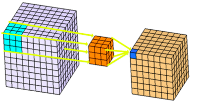
This is achieved through the use of filters (often called kernels in the literature). A filter is a small weight matrix (e.g., 3×3, 5×5) that slides over the image and performs a convolution operation (Visual Example). If you are a mathematician, you might say: "Hey, but this is actually cross-correlation, not convolution!" – and you would be correct. In cross-correlation, the signal (or filter) is not flipped. However, in practice, we usually call it convolution because the learning algorithm can adjust the filter weights if flipping is necessary. In this sense, calling it convolution is a more general statement. The reduced number of parameters also benefits the learning process, making the network more resistant to overfitting (given a sufficiently large dataset) and allowing it to learn faster. Additionally, these networks generalize better and require less training data than classical neural networks to achieve higher accuracy.
 https://arxiv.org/pdf/2010.08515
This stems from the built-in inductive bias – in convolutional networks, filters learn to detect local patterns (e.g., edges, corners), and successive layers combine these features into increasingly complex structures. As a result, the network assumes certain properties of images – locality, translational invariance, and weight sharing – instead of learning them from scratch.
Convolution: The Mathematical Operation Behind CNNs
The convolution operation in mathematics is defined as follows (continuous case):
$$ (f * g)(t) = \int_{-\infty}^{\infty} f(\tau) , g(t - \tau) , d\tau $$
which is interpreted as:
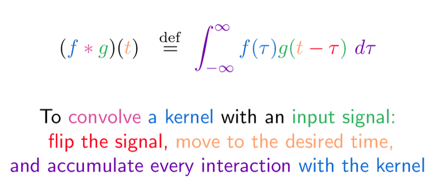 https://betterexplained.com/articles/intuitive-convolution/
In the discrete case, such as when processing images, the convolution is defined as: $$ S(i, j) = (I * K)(i, j) = \sum_m \sum_n I(i - m, j - n) , K(m, n) $$
Where:
- pixel value of the input image at position (i, j): $$ I(i, j) $$
- value of the filter (kernel) at position (m, n): $$ K(m, n) $$
- resulting pixel value in the output feature map: $$ S(i, j) $$
To better understand this operation in depth, I recommend the following link: 3Blue1Brown - But what is a convolution? starting at 6:30.
Example of a CNN
In practice, a single convolutional layer typically uses more than one filter. The resulting feature maps from each filter are stacked together and passed to the next layers. At the end, all feature maps are often flattened into a single vector, which serves as the input to a fully connected neural network. Additionally, for example, in classification tasks, the final layer usually applies the softmax function to produce class probabilities.
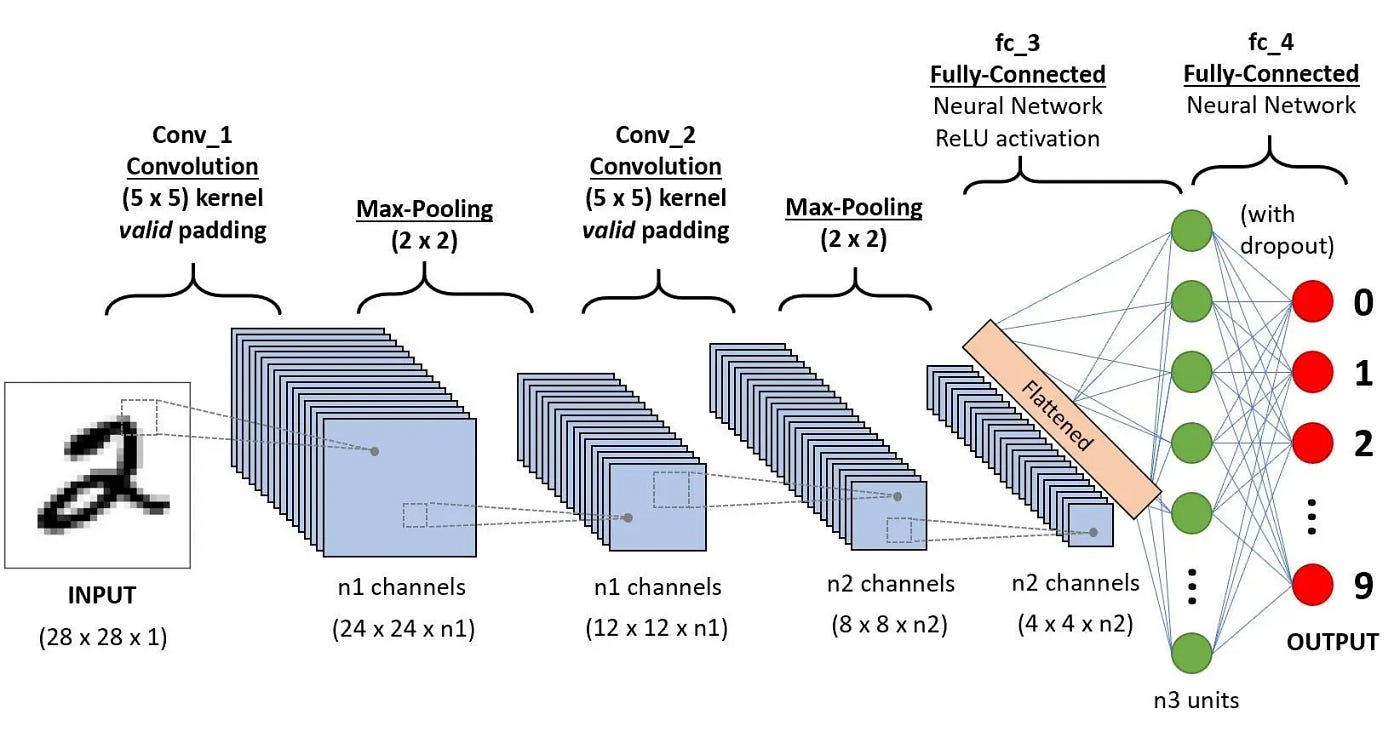
At this point, let's pause to explain a few things. Padding means adding extra pixels on each side of the input (if you imagine a framed picture, the frame is essentially the padding). Padding helps us preserve more information at the borders of an image. Without padding, only a few values in the next layer would be influenced by pixels at the edges. It also allows us to maintain the original input size of the image. The output size is given by the following formula: $$ H_\text{out} = \left\lfloor \frac{H - F + 2P}{S} \right\rfloor + 1 $$ $$ W_\text{out} = \left\lfloor \frac{W - F + 2P}{S} \right\rfloor + 1 $$
Where:
- H – height of the input image
- W – width of the input image
- P – padding (border with values usually set to 0)
- S – stride (instead of moving the filter by 1, we move it by S pixels)
In short: we first compute the total dimension of the input matrix including padding and treat this as our effective input. Then we subtract the filter size (this gives the number of positions the filter can move by 1 in the remaining space), divide by the stride S (we skip every S-th position), and finally add 1 (remember that the filter starts at the top-left corner).
Padding can be either:
- valid – no padding (output size is smaller than the input)
- same – padding is applied so that the output has the same size as the input
Max-Pooling works on the same principle as a sliding window, but it performs a different operation – it takes the maximum value within the window. As a result, there are no learnable parameters in this layer. Besides max-pooling, there is also average-pooling, which computes the arithmetic mean of all elements in the window. They are used to reduce the size of the input and help make feature detectors more invariant to the features’ positions within the input.
Flatten combines the input into a single vector of numbers, converting multi-dimensional data (like feature maps) into a one-dimensional array for the next layer, typically a fully connected (dense) layer.
Dropout is a regularization technique used to prevent overfitting in neural networks. During training, it randomly "drops" a fraction of neurons (sets their output to zero) in a layer for each forward pass. This forces the network to not rely too heavily on any single neuron and helps it generalize better to new data.
CNN Learning
Learning convolutional neural networks follows the classic neural network training process, with the key difference that the network learns filter weights that detect patterns in images. The goal is to find a set of weights that ensures the network’s output closely matches the desired output for each input. Below is a step-by-step overview of the learning process of a convolutional neural network (CNN):
-
Forward pass
- The input image passes through convolutional and pooling layers.
- Each filter detects characteristic patterns (e.g., edges, corners).
- At the end of the network (often after flattening and fully connected layers), we get a prediction.
-
Loss computation
- The prediction is compared to the true label (e.g., image class).
- A loss function (e.g., cross-entropy for classification) measures how wrong the network is.
-
Backward pass (backpropagation)
- Gradients of the loss function with respect to the filter weights are computed.
- The network learns which features are important for correct classification.
-
Weight update
- Filter weights are updated using an optimization method (e.g., Stochastic Gradient Descent, Adam).
- This allows filters to better detect patterns in images over time.
-
Repeat
- Steps 1–4 are repeated for many images and training epochs.
- Over time, the network learns to generalize patterns better and classify new images correctly.
This is a challenging topic, especially backpropagation, which requires three key components: a dataset, a feedforward method, and a cost function. I encourage you to look for more information about it online.
It is also worth knowing that each layer, whether convolutional or pooling, has its own way of computing its output. Connections within a layer or from higher to lower layers are not allowed, although skipping intermediate layers is possible. Moreover, any input-output function with a bounded derivative can be used, but combining inputs linearly before applying a nonlinearity makes learning much simpler.
Summary
Convolutional neural networks (CNNs) are a complex topic and take time to fully grasp. I hope that, at least to some extent, I’ve been able to introduce you to the subject and explain the key concepts. If you want to try working with them in code, I encourage you to take a look at my notebook: Sign Language Image Classification