Introduction

If you’ve read my post about the autocorrect system, you might remember the promise I made back then:

In a future post, I’ll go into more detail about dynamic programming.

I always keep my promises (which is why I make them so rarely :) ), so today’s post is all about dynamic programming.

If you’ve been around computer science for a while, you’ve probably heard about programming paradigms like object-oriented or functional programming. The term dynamic programming might sound similar, but it actually refers to something quite different. Dynamic programming is a method of solving problems by breaking them down into smaller subproblems and using the results of already-solved subproblems to build up solutions to larger ones.

In simple terms, you can think of it like designing a user interface: the whole app is the main problem, and the subproblems are the individual UI components — buttons, forms, info cards, and so on. You combine these smaller parts into bigger sections of the interface, then into full pages, and eventually, you get a complete app. Notice that to build the whole application, you first need to create a few larger sections of the UI (like a navigation bar, content panel, and footer). And to build each of those sections, you reuse smaller, previously designed components.

That’s the key idea — when designing each new piece of the UI, you’re relying on ready-made building blocks you’ve already created.

This explains when to use dynamic programming: when there’s overlap between subproblems — that is, when the same smaller subproblems appear multiple times while constructing the full solution. By solving and storing those smaller pieces, you can gradually build up the final answer without repeating work.

If, on the other hand, a problem can be solved by combining the results of non-overlapping subproblems, that approach is called divide and conquer. In app design terms: if every section of your app uses completely unique elements (each one has its own distinct buttons, forms, etc.), then that’s divide and conquer, not dynamic programming!

Problem-Solving Techniques in Dynamic Programming

All problems that can be solved using dynamic programming are handled using one of the following approaches:

• Top-down approach
• Bottom-up approach

These are simply different ways of organizing the computations — deciding how to solve subproblems and in what order.

In the bottom-up approach, you start from the smallest, simplest pieces and then combine them step by step into larger and larger parts (just like in the analogy above).

The top-down approach (also known as recursion with memoization) works the other way around — you start from the overall problem and gradually break it down into smaller subproblems.

In the context of UI design, you can think of it like this: first, you sketch out the entire view of your app, and then you figure out which components it’s made of. You create each element (like a login form, buttons, or text fields) only when it’s needed — and if a component appears again somewhere else in the app, you reuse the version you’ve already built instead of making it from scratch.

Theory in Practice

Let’s get back to the topic of our simple autocorrect system.
The goal of autocorrect (for those unfamiliar) is to find a word from a given dictionary that best matches the word the user typed incorrectly — usually, it’s the one that can be obtained with the smallest number of letter changes. For example, let’s say our dictionary looks like this:

dictionary = ["dog", "bike", "book"]

and the user typed the word buuk on their phone. To turn buuk into dog, we need to perform 4 operations:

1. change b → d
2. change u → o
3. change u → g
4. delete k

Of course, there are many other possibilities — some optimal, some not.

For bike, we need 3 operations:

1. change u → i
2. change u → k
3. change k → e

For book, we need only 2 operations:

1. change u → o
2. change u → o

So, the most likely word the user meant to type is book.
(In real autocorrect systems it’s not quite that simple, but older systems actually worked in a very similar way)

Now, let’s think about how to write a program that returns the minimum number of insertions, deletions, or substitutions (where a substitution counts as one operation, even though it’s technically a delete + insert).

To visualize this, let’s draw a table like this:

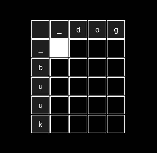
Where:

• The first column contains the word entered by the user
• The first row contains the word we’re comparing it to (the target)
• An extra empty row and column are added at the start to make a “starting point” (the white cell) for the algorithm — this simplifies the code
• We start with the word on the left (in memory)
• We can only move right or down:
• Moving right means inserting a character from the top word (at column index j)
• Moving down means deleting a character from the left word (at row index i)
• Each pair of different moves is treated as one operation — the system checks whether the insert + delete combo was meant to replace a character (1 operation, not 2), or if the characters were actually the same (in which case, there’s no edit at all).

By checking all possible paths from the top-left corner to the bottom-right corner — and picking the one with the smallest total cost — we get the solution to our problem:

For the two words above, the smallest number of edits we get is 4.
Notice that we pass through many of the same cells multiple times, which means we waste a lot of time recalculating the same values.
The time complexity of this algorithm is:

$$ O\left(\binom{m+n}{m}\right) $$

Where:

• m – the number of rows
• n – the number of columns

This complexity grows very quickly for large values of m and n.
Now, let’s look at an approach that uses dynamic programming, where the time complexity is:

$$ O(m \cdot n) $$

We’ll use the bottom-up approach — starting with the smallest substrings and building up solutions for larger ones. The trick is that we store the minimum edit distances for all substring pairs in a table, so we don’t have to go through the same cells multiple times.

To simplify the algorithm, we’ll fill the first row and first column with values representing the number of insertions and deletions needed:

• the first row shows how many insertions are required to go from an empty string _ to the top word up to index j,
• and the first column shows how many deletions are needed to go from the left word down to index i, ending with an empty string _.

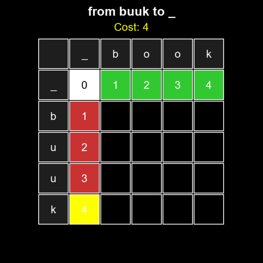
Now, for each of the remaining empty cells, we simply run our VAR system, but with a slight modification. That’s because we can reach a given cell not only through two consecutive different moves, but also through a sequence of the same moves — for example, three insertions if we’re in the fifth cell of the first row (a cell with a cost of 4). So, what we do is:

• If the characters at the current positions are the same, the cost is simply the value from cell [i-1][j-1]
• Otherwise, we look for the cell we could have come from with the smallest cost and add 1 (the cost of substitution)

The code for our system would look like this:

    for i in range(1, n):
        for j in range(1, m):
            if s1[i - 1] == s2[j - 1]:
                matrix[i][j] = matrix[i - 1][j - 1]  # Characters are the same, no operation needed
            else:
                matrix[i][j] = min(
                    matrix[i - 1][j] + 1,
                    matrix[i][j - 1] + 1,
                    matrix[i - 1][j - 1] + 1
                )

The entire process of how this algorithm works is shown below:

In the top-down approach, we start with the main problem: “how many operations are needed to transform buuk into book?” and then we divide it into three subproblems:

1. How many operations are needed to transform buuk → boo
2. How many operations are needed to transform buu → book
3. How many operations are needed to transform buu → boo

Each of these subproblems is then divided in the same way, until we reach one of the base cases:

• First word is empty
• Second word is empty

Additionally, if at any point during the algorithm the characters being compared are the same, we can skip two subproblems using the following logic:

if word1[i - 1] == word2[j - 1]:
    return levenshtein(word1, word2, i - 1, j - 1)

Visualizing the recursive approach isn’t as neat as the iterative one, so I’m skipping it here. This algorithm essentially explores the table in a tree-like manner, but because of the order in which the recursive calls are made, it ends up looking pretty chaotic.

Code for Both Approaches

Below, I’m sharing the code for both methods:

1. Bottom-up

def levenshtein_distance(s1, s2):
    # s1 = source, s2 = target
    n = len(s1) + 1  # add an empty character at the beginning of s1
    m = len(s2) + 1  # add an empty character at the beginning of s2
    matrix = np.zeros((n, m), dtype=int)

    # The two loops below are used so that we don't have to check bounds in the main loop.
    # The number of operations needed to convert s1[:i] to an empty string (i.e., deletions)
    for i in range(n):
        matrix[i][0] = i

    # The number of operations needed to convert an empty string to s2[:j] (i.e., insertions)
    for j in range(m):
        matrix[0][j] = j

    # Compute the Levenshtein distance
    for i in range(1, n):
        for j in range(1, m):
            if s1[i - 1] == s2[j - 1]:
                matrix[i][j] = matrix[i - 1][j - 1]  # Characters are the same, no operation needed
            else:
                matrix[i][j] = min(
                    matrix[i - 1][j] + 1,
                    matrix[i][j - 1] + 1,
                    matrix[i - 1][j - 1] + 1
                )

    return matrix[n - 1][m - 1]

2. Top-down

def levenshtein_distance(s1, s2, m, n):
    # First string is empty
    if m == 0:
        return n

    # Second string is empty
    if n == 0:
        return m

    # Skip the other two subproblems
    if s1[m - 1] == s2[n - 1]:
        return levenshtein_distance(s1, s2, m - 1, n - 1)

    return 1 + min(levenshtein_distance(s1, s2, m, n - 1),
                   levenshtein_distance(s1, s2, m - 1, n),
                   levenshtein_distance(s1, s2, m - 1, n - 1))

Summary

As shown earlier, using dynamic programming can significantly speed up your program by storing and reusing the results of previously solved subproblems. Dynamic programming is typically used when a problem (technically speaking) involves overlapping subproblems — situations where certain computations are repeated and can therefore be cached — and an optimal substructure, meaning that the solution to a large problem can be built from the best solutions to its smaller parts.

When you encounter a problem that might be solvable using DP, it’s worth asking yourself the following questions:

• What does each dimension and each cell in the table represent (in the case of a bottom-up approach)?
• What are the smallest subproblems that I can later combine into larger ones?

I hope I managed to give you a clearer idea of what dynamic programming is and why it’s worth using whenever possible. I also encourage you to keep exploring the topic — there are many optimization techniques out there, including ones that reduce the space complexity of DP algorithms.

See you in the next post!

References

https://en.wikipedia.org/wiki/Dynamic_programming

NEURAVERS - Simple Autocorrect System